Astronomical Techniques - Spectroscopy
Objective: accurate determination of the energy distribution of radiation
from distant objects as received above the atmosphere, free of
instrumental and atmospheric effects. Ideally, all incident
photons should be collected and used (DQE=100%). Applications
of spectroscopy are the backbone of astrophysics, probing both
the conditions of emission of radiation and its modification en
route to the observer. Spectroscopy is possible by appropriate
techniques in all wavelength regimes.
There are several basic approaches:
Dispersive: convert wavelength to one detector coordinate, so
we really measure x,y and infer x,λ.
Nondispersive: measure or reject photons in a way that relies
directly on wavelength. Optical applications so far are mostly in
narrowband imaging (such as in Fabry-Perot devices, some of which are
tunable over wide wavelength ranges, or tunable circular filters). These
techniques are very effective at high energies and in the radio
regime. A particularly elegant application, especially useful in the
infrared, is the Fourier transform spectrometer. In Jim Brault's
description, these are the concrete embodiments in glass and steel
of Fourier's equation.
Spectroscopy requires particular considerations for instruments and detectors:
Efficiency: dispersion reduces photon flux compared to broad-
band imaging, so the requirement here is more exacting. Likewise,
detector background and bias patterns are more of a problem for
spectroscopy than broadband imaging.
Dynamic range: (perhaps including foreground sky lines as well
as any strong lines from the target)
Resolution (spectral and spatial)
Scattering (aliasing radiation into false frequencies)
Stability and calibration accuracy
Background - dark current and readout noise,
worse problems than for imaging
Spectroscopy versus spectrophotometry
Dispersive spectrographs:
Prisms
Gratings, echelle versions
Grisms (grating prisms)
Normally, we use a sequence of collimator-disperser-camera. Clever use
of curved gratings (as in the Rowland circle) or double-pass
optical systems can eliminate one of
these. In Littrow-type designs, the grating also collimates or focuses.
Comparison of dispersive elements:
Prisms: two surfaces, absorbing glass may become thick. Wavelength
dispersion is highly nonlinear; frequency dispersion more nearly linear,
set by index of refraction of prism material. Slitless spectroscopy
can use thin objective prisms (since light is
also parallel before entering the telescope). Prisms are used in,
for example, STIS, as fallback elements for very deep reconnaissance
spectra at low resolution.
Reflection) gratings: one reflection, dispersion uniform in wavelength.
May
have groove shape set for high efficiency at certain wavelengths (blazed).
Various orders may overlap, since angular dispersion is set by the grating
equation d (sin i + sin θ) = m λ
where m=order number; reduces to d sin θ at normal incidence.
Multiple orders may be a disadvantage, requiring cross-dispersers or
filters to reject unwanted wavelengths, or an advantage, allowing multiple
wavelength ranges to be observed (as in echelle spectroscopy). The
theoretical resolution of a spectrograph increases proportionally to
the number of grooves
illuminated by the beam, but in astronomy it is more usually limited by the
slit or aperture size.
Periodic errors in groove spacing lead to ``ghost" images of spectral lines.
The ruling may be scribed by a mechanical image, produced by holography and
photosensitive etching, or made by replication from a master made in these ways.
Transmission gratings may be used in front of an objective or near the focus
(preferably in a parallel beam). Zero-order (nondispersed)
images sometimes cause trouble with dynamic range or confusion, at other
times can be useful for wavelength calibration (especially for
slitless spectroscopy).
Grisms (grating/prisms): transmission grating ruled on a thin prism, with
deviations cancelling at the undeviated central wavelength. This allows a
stright-through optical system (mechanical and optical advantages), plus
higher throughput at moderate dispersion than reflection grating. Grisms
are the heart of the current generation of high-efficiency spectrographs
(Cryogenic Camera at KPNO, EFOSC at ESO, Faint-Object Spectrographs at La
Palma, applications on HST). A high-order version has been used at Lick
(the "echism"). This compares to a traditional echelle grating,
one blazed for best efficiency in a high order, used on a range of
high orders n ~ 20 with cross-disperser to stack the orders
on a 2D detector, thus combining spectral range and high dispersion.
Considering optical elements in the order traced by the light path:
Focal plane
may be open (for slitless work), with high sky background but very
wide field for surveys;
apertures, for spectrophotometry or multiobject work (slitlets,
holes, arcs to follow gravitational lenses),
slit (to avoid spectral overlap, unnecessary sky background). Can
tilt the slit so it's not quite perpendicular to the incoming beam,
and aluminize its surroundings so that a reflected image is
visible for acquisition and guiding. Slit length and open region may be
defined by use of a so-called decker plate (dekker in Britain), to
block bright objects or excessive sky light and sometimes allow
interesting tricks in moving the spectrum along the slit.
Or finally fibers: may be a fixed array (Dense-Pak, TIGER, MPFS, GMOS IFU)
or moveable (Hydra, Argus,
MX, Nessie, FLAIR, 2dF...) for desired object positions. Some fiber arrays use
multipupil reimaging systems (which can also work directly into a
spectrograph, as in Tigre at the CFHT). Internal reflections near the fiber
tip decrease the output focal ratio, which must be taken into account in
spectrograph design to avoid light loss.
Filters: for order blocking, sometimes allegedly neutral (gray) ones for
control of calibration or standard-star intensity. Beware of tilted filter
producing wavelength shifts below the slit. May also help in baffling stray
light; such baffling is critical in spectrograph design, since light goes
anywhere it can whether you want it to or not. A particular issue
is that undispersed scattered light can swamp the dispersed light that you want.
Collimator: most dispersing elements (such as plane gratings, prisms, or
grisms) work properly only in a parallel beam. The collimator should match
the incoming focal ratio (possibly after modification by fibers), and the
beam size at the disperser. Frequently an achromatic lens or concave
mirror, best used off-axis to avoid light loss.
Dispersing element: may need to have adjustable tilt, or be changeable during
observations. The accuracy of repositioning is important in efficiency,
as to which calibrations must be repeated after moving and resetting it.
Camera: focuses the parallel beams of dispersed light onto the
detector. To
match the detector image scale and scale of telescope vs. seeing, this may
be very fast (f/0.8 isn't unusual), so folded Schmidt designs are common.
Fast well-corrected lens sets may also be used. In some cases, the camera
is built into the dewar housing a cooled detector.
The geometry of all these may be strongly folded, and may have focussing
aids such as Hartmann masks included. There may also be provision to view
from behind the slit for centering and guiding, either visually or with a
low-light TV camera. Some loss in light occurs during folding (even
0.95n
can become small). Large fixed spectrographs may be used to avoid excess mirrors
(even though Coude' light paths usually have 3-5 mirrors anyway).
Some samples of a traditional grating spectrograph and a compact
grism-based imager/spectrograph illustrate the range of possible designs.
Detectors:
People actually started out doing astronomical spectroscopy by eye.
I'm impressed. But the eye
is non-recording and non-integrating.
Photographic emulsions (hypersensitized or not) - special spectroscopic
emulsions optimized for long exposures without reciprocity failure. Easy to
use, portable, no support equipment needed, come in very large formats. On
the other hand, their DQE is low (almost always < 1%), they are quite
nonlinear in response and painful to calibrate, and grain irregularities
cannot be calibrated. They store their own results without magnetic media,
though. Sometimes used with image intensifiers to increase DQE and evenness
of spectral response (at the expense of introducing spatial structure due
to the internal cathodes, limiting S/N with any detector). These may also
produce temperature-dependent geometric distortions. Trailing of stellar spectra can be used to increase
S/N ratio, by averaging across larger numbers of grains on the emulsion.
Electronographic emulsions: record photoelectrons from a cathode rather
than photons. Can be very sensitive, have higher dynamic range than direct
plates. Also fantastically finicky and difficult to use.
Photomultipliers: one- or few-channel systems, for highest
spectrophotometric accuracy or in otherwise inaccessible wavelength
regions. Very accurate and sensitive, but there can be only a limited
number of channels so that a slow array beats a fast PMT. Use with a moving
grating or circular variable filter (CVF). No two-dimensional capability.
Everybody once had to do it this way in the infrared.
Discrete-aperture systems} (one-dimensional use of detectors; now
largely historical)
IIDS (Intensified Image-Dissector Scanner): a hybrid system with three-stage
image tubes, and the final output
phosphor scanned rapidly (on the decay time scale of each photon's output
flash) along spectral traces of two apertures by an image dissector,
magnetically scanned into a photomultiplier. Description by Robinson and
Wampler 1972, PASP 84, 161.
Almost exactly linear (some
applications have output = const X input1.03, for example). S/N limited
to 100 or so by instabilities in exact location of output spectra, so that
the flat-field correction changes. At high count rates, a coincidence
correction is needed (as with true photon-counting systems). These systems
(Lick, AAT, KPNO, ESO) have been widely used for surveys of stars, QSOs,
galactic nuclei. The readout is visible in real time. Dual apertures serve
for simultaneous sky subtraction or (for large objects) simultaneous
measurement of two position and time-switched sky subtraction. Polarimetric
operation is possible by scanning four spectral traces, one from each
aperture as split into polarization senses by calcite blocks (Miller,
Robinson, and Schmidt 1980, PASP 92, 702).
Adjacent pixels are not truly independent, since each photon flash has
nonzero width (clever software could improve this), so S/N statistics are
not trivial to work out.
Reticons (with or without intensifiers): 1-d arrays (as used in store
checkout lines) typically having 1024 diodes, having internal connections
for self-scanning readout. This introduces 2,4,8,16...-channel
fixed-pattern noise (removable by bias observations). The readout noise
tends to be rather high, but the electron capacity of each diode is huge.
This allows observations of bright targets at S/N up to 1000.
Relatives of these also exist, such as the HST-FOS Digicons.
Panoramic detectors:
SIT (Silicon-Intensified Target) tubes: integrating TV cameras, used in a
charge-storage mode or constantly read out in an "equilibrium" mode. The
dynamic range in direct mode is quite limited by changes in the flat-field
pattern, as is the S/N achievable. Use of photon-counting
(event-centroiding) electronics as in the IPCS remedies some of this. The
preparation time for each exposure is long (up to 15 minutes) since each
part of the camera tube must be cleared of accumulated charge. Readout can
be similarly lengthy, passing an electron beam across the faceplate and
recording the resulting current. This may suffer from beam-pulling effects.
Vidicons of this kind were used on IUE.
IPCS (Image Photon-Counting System): uses TV or related CCD system and
fast centroiding electronics to give position and time of each detected photon,
accumulated in real time into a display memory. Has very low (essentially
zero) "readout noise", and is thus most effective at high dispersions and
low photon rate, where CCD readout noise overwhelms the higher DQE of CCDs.
Large numbers of pixels (2048 by 100) are possible. Relatives: KPCA,
2-D Frutti.
MAMA (Multi-Anode Microchannel Array): microchannel plate feeding a
multi-anode array that times individual electron bursts; acts as a photon
counter. These are especially useful in the ultraviolet, where they retain
high efficiency. The cathode can be designed with a work function
(as in the relation KE = h ν - W) such that zero electrons
are liberated by photons of wavelength longer than a certain cutoff,
resulting in a "solar-blind" detector. Since scattered sun- and star-light
can swamp weak UV signals, even within a baffled spectrograph, this
is a much-prized feature. As photon counters, MAMAs have count-rate
limits, first related to deadtime correction, then to device safety.
They also may have a cumulative count limit (example: FUSE sensitivity
at wavelengths of geocoronal H emission decreased rapidly, bright targets
being put off until late in mission).
CCD (Charge-Coupled Device): the current observers' darling. See C. MacKay
1986, Ann Rev 24,255 and various observatory newsletters. Solid-state array
of potential wells (in fixed pixel array), in which changes in clock
voltages can move charge around and eventually through an on-chip amplifier
and thence to the outside world. Pixel sensitivities nonuniform but usually
flatten to better than 1%. Excellent stability with time, linearity, DQE up
to 90% in some spectral ranges. Readout noise usually the limiting factor.
Thin/thick chips, red/blue sensitivity, blue enhancements by UV flooding or
coatings, cosmic-ray sensitivity.
Formats up to 2048 by 4096 exist.
Fringing in spectroscopic applications, especially in deep red, from interference
of internally reflected light.
On-chip binning is sometimes useful for readout noise and dynamic range
improvement when loss of spatial sampling can be tolerated.
Bias and charge-transfer efficiency, preflashing.
Cosmetic defects in imaging/spectroscopic applications.
Can be read in analog mode (TV rates) for guiding or (with intensifier) for
a pseudo-photon counter (2D-Frutti, KPCA).
Behavior at/near saturation.
ADUs versus photons and noise calculations.
S/N in instrument comparisons and exposure calculations; sometimes a less
sensitive detector will give better results.
Infrared Arrays began life as both tactical and strategic sensors
for the military. They use variously doped compounds (InSb, GaAs)
and direct readout. Unlike CCDs, each pixel can be read directly
and can be read repeatedly in a nondestructive way, allowing reduction
in readout noise. These normally have to be read frequently, since
the thermal background from ground-based sites would saturate the
detector quickly all by itself (a minute or two at K, milliseconds
in the 5 μ band), which led to the development of very fast
electronic setups. Likewise, sky subtraction is the big deal
in reduction, followed by mosaicking of many small partially-overlapping
frames. IR arrays lagged behind CCDs in format, with 256 X 256
detectors on NICMOS. By now there are a few usable 10242 arrays.
At high count rates they require correction for nonlinearity.
REDUCTION PROCEDURES (generic for two-dimensional linear detectors);
relevant IRAF procedures are in [brackets]
1. Internal detector properties (as for imaging)
Bias pattern: subtract average bias pattern from large number of zero-time
exposures.
Bias level (changes in DC offset of CCD amplifier): form average row or
column of overscale region, subtract from whole frame. Usually trim edge
pixels off at this stage to avoid blowups.
[noao.imred.bias.(colbias/linebias)]
Preflash: if nonuniform, may need to subtract average or scaled
long-exposure preflash from raw data.
Dark pattern: subtract scaled dark frame (which has itself been bias-corrected),
as scaled to the actual exposure time. For "warm" systems such as our
SBIG cameras, dark subtraction is really important. The dark frame
may not be quite linear with expowsure time, so it's important to
get darks with the same exposure time and chip temperature as the
data exposures. With these systems, the bias drifts usually corrected
using the overscan region should be swallowed
up in the bias-frame subtraction.
2. Detector response:
Flatten flat-field exposure in the dispersion direction
(since you're not interested in the wavelength
distribution of the flat-field lamp), by some smoothing algorithm along the
relevant axis.
[noao.imred.generic.flat1d]
Normalize this, and divide data with the same grating setting/wavelength
range. Different flats must be obtained for each wavelength range, since
pixels have different wavelength sensitivity over large ranges
(manufacturing irregularities) and small (fringing).
3. Determine coordinate-wavelength mapping:
Need to have observed a wavelength standard, usually an internal
emission-line lamp (though in a pinch night-sky emission or a bright
planetary nebula can be used in the red and near-infrared).
Measure the pixel coordinates of emission features and fit some useful
function for interpolation (typically some set of orthonormal polynomials
or ordinary polynomials). It may be necessary to do this in the
perpendicular direction as well, using stellar or special calibration
images, to map optical distortions or atmospheric dispersion.
[twodspec.longslit.identify, reidentify]
For most applications, the fit generated from these calibrations will be
sued to rebin the two-dimensional spectrum onto linear wavelength and
spatial scales.
[twodspec.longslit.fitcoords, transform]
Be careful with order of interpolation and quality of sky subtraction here.
For high-precision radial velocity work, frequent wavelength calibrations
are done at the same telescope positions. Particularly for grating
spectrographs, engineering considerations for flexure control
are paramount. The odd shape required by multiple off-axis reflections,
perhaps with folding mirrors, can make this control very tricky. The
highest accuracy, as needed for extrasolar planet searches, uses
an iodine cell in the beam to superimpose many narrow absorption lines into the
object spectrum, and also requires detailed accounting of slight asymmetry
in the final line profile.
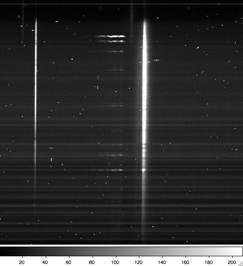
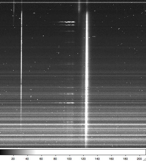
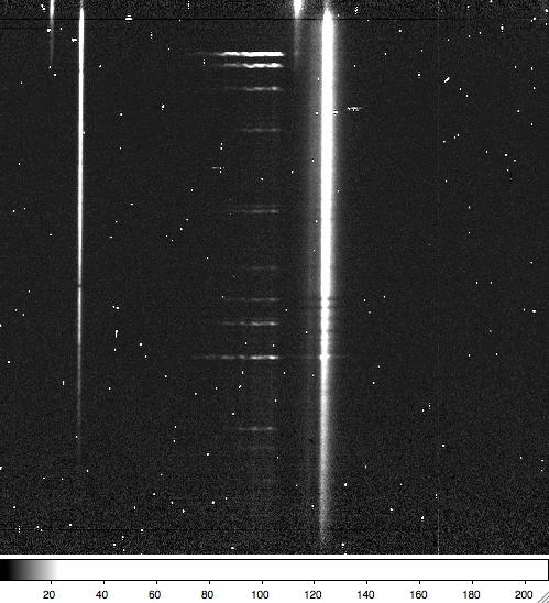
4. Subtract the foreground night-sky emission
Particularly in the red, OH emission makes a forest of the blank-sky
spectrum (sometimes useful for secondary wavelength calibration).
For space data, the major contributors are scattered sunlight from dust in
the inner solar system, scattered starlight from interstellar grains, and
Lyman α emission from the geocorona.
Subtraction may use interpolation or some kind of averaging. It is
sometimes necessary to use a blank-sky spectrum to correct for nonuniform
illumination along the slit at this stage.
[noao.imred.generic.background]
Night-sky emission becomes terrifying
for λ > 6600 Å. Lists of airglow emission lines are given in
Broadfoot and Kendall, J. Geophys. Res. 73, 246 (1968) and Krassovsky et
al., Planetary Space Sci. 9, 883 (1962).
An improvement has been worked out by Kelson (2003 PASP 115, 688), in
which one uses the 2D location/dispersion solution to identify the
exact wavelength of each pixel, and derive the mean sky for a
wavelength grid sampled at subpixel intervals. This obviates the
need to interpolate crudely-sampled sky features, which can otherwise
induce "ringing" in the subtracted spectrum, and come much closer to
Poisson statistics throughout the spectrum.
Another improvement is the nod-and-shuffle technique, in which the
spectrum is limited to 1/3 the total CCD size. In this case, the telescope
is nodded to new positions along the slit asthe charge is shuffled a
matching range on the detector, so one ends up with two sky spectra
of the same total exposure and same mean time of observation, observed
through the same optical path, as the object. This has been very successful
in taming the near-IR OH airglow bands (as in the Gemini Deep Deep Survey,
chasing weak absorption lines into the near-IR). One almost always
ends up doing some similar shuffling for near-IR spectra, where the
sky lines are stronger and more numerous.
5. (optional for some purposes) Absolute flux calibration
Uses a standard star. After doing all of the above, extract a standard star to
one-dimensional form, and compute the flux corresponding to one ADU or
other instrumental unit, either assuming the wavelength dependence of
atmospheric extinction or measuring it from multiple standards. This gets
less and less well determined for narrower slits, since that becomes more
sensitive to changes in seeing or guiding errors. Standard stars are also
used to derive corrections for telluric absorption features due mostly to
O2 and water vapor (particularly in the red, huge in the infrared).
[proto.toonedspec],
[onedspec.standard,response,calibrate]
Atmospheric effects can also enter here through differential refraction -
the atmosphere acts as a thin prism. For large wavelength ranges,
a small aperture cannot simultaneously encompass the object in all
wavelengths without some compensation device. The most commonly encountered
(and not too often at that) is a set of Risley prisms - two rotating
thin prisms which can be set to give a desired total dispersion and
direction. Appropriate glasses can do a fair job of dispersion compensation.
The relevant formulae for dispersion are given by Filippenko 1982 (PASP
94, 715) along with useful tables and graphical examples. When possible,
this problem can be circumvented by placing the spectrograph slit vertically,
but this is not always possible if a particular orientation is important
across the object.
6. Measuring wavelengths, line ratios, equivalent widths, redshifts by
correlation techniques. Redshifts via cz, c β,
corrections for
terrestrial and solar motions.
« Photometry |
Astrometry »
Course home page |
Bill Keel's Home Page |
Image Usage and Copyright Info |
UA Astronomy
keel@bildad.astr.ua.edu
2006 © 2000-2006