Observational selection effects must first be understood when they cannot be eradicated. The foremost example is Malmquist bias, the fact that in a typical flux-limited sample we see only atypically bright objects at larger distances. This is a major fact of life in extragalactic astronomy; as Trimble (1996, PASP 108, 1073) points out, "Any large gathering of observational cosmologists today will include at least one person who thinks that someone else in the room does not understand the Malmquist effect". To allow for this effect, we need to know or guess the luminosity function (LF). As a simple example, take a class of objects with a uniform spatial distribution and a Gaussian LF; extreme values only occur within large volumes and thus at large distances, and the detection threshold (slanting line in the picture, where we detect only objects above it) means that the mean luminosity of the sample grows with distance even if the population does not change at all. The situation will look like this:
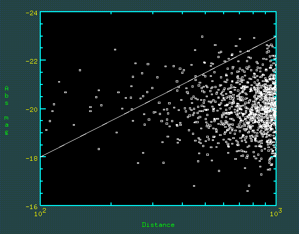
For real galaxies the situation is even worse, because the LF is very steep and very deep; this is why we don't know much about the population of dwarf galaxies. It is always safe (but seldom possible) to search much deeper than you might need to - otherwise elaborate statistical manipulations, such as survival analysis, will be needed to reconstruct the true properties of the sample distribution. Clusters of galaxies are popular for studies of the luminosity function for the same reason that star clusters are - distance-dependent effects are usually insignificant within a single cluster, so that the galaxy population in the cluster may be evaluated free of Malmquist bias. However, using clusters at a range of distances suffers not only from the Malmquist bias, but from the Scott effect - the fact that to be recognized as such at great distances, clusters become less and less typical in population. Note also all the selection effects mentioned at the outset of the course - surface brightness and compactness limits - mean that some kinds of galaxies are barely represented in existing catalogs. These selection effects are especially damaging for distance-scale problems.
The number of galaxies of various Hubble types in a magnitude-limited sample is typified by these numbers from the RSA catalog:
| Ordinary | Barred | ||
| E+E/S0 | 173 | SB0+SB0/Sba | 48 |
| S0+S0/a | 142 | SBa+SBab | 42 |
| Sa+Sab | 123 | SBb+SBbc | 96 |
| Sb+Sbc | 187 | SBc | 77 |
| Sc | 293 | SBcd+SBd | 8 |
| Scd+Sd | 26 | SBm+IBm | 9 |
| Sm+Im | 13 | ... | ... |
| S | 16 | ... | ... |
| Special | 18 | ... | ... |
| Totals | 991 | ... | 285 |
Types Sd,Sm are underrepresented in this flux-limited compilation because they are intrinsically fainter than the earlier spiral classes Sa-Sc. Some ellipticals (the sequence continuing into dwarfs) have similar problems. Only the types S0-Sc are probably fairly represented - these are giant galaxies and can be seen at large distances. If we regard Hubble type as mapping a continuous structural variable, the number of galaxies tells us about the bin widths of the Hubble classes in this variable.
Correlations with Hubble type may be examined in detail by using de Vaucouleurs' type index T, assigned as follows:
| Type | E | E/S0 | S0 | Sa | Sb | Sc | Sd | Im |
| T | -4 | -2 | 0 | 1 | 3 | 5 | 7 | 10 |
A further luminosity-class index L (ranging 1-5) is defined for spirals and irregulars. The joint distribution of these for galaxies in the RC2 is given by de Vaucouleurs 1977 (Evolution of Galaxies and Stellar Populations, p. 43). Many useful quantities correlate with T, as shown in his Fig. 2.
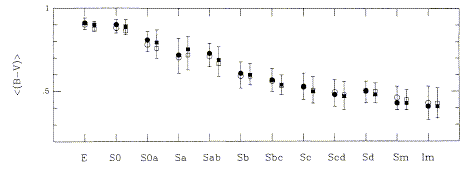
Later-type galaxies are fainter in the mean - the scatter is quite large. Note that corrections for internal extinction needed to be made. As well as total optical luminosity and H I content, optical spectra and therefore color indices that relate to SFR history change with Hubble type. Some well-known examples are the UBV system indices U-B,B-V. These three passbands are centered near 3500, 4300, and 5800 Angstroms with passband widths 600-1400 Angstroms. Fig. 6 from de Vaucouleurs 1977 shows their variation (integrated across the whole galaxy) with T.
Early types E/S0 have red colors, as expected for systems with very low SFR. Later types have bluer colors, indicating a larger relative rate of recent star formation. This test alone does not tell whether this is due only to bulge/disk variations, chemical abundance effects or a real difference in the disk histories (I recall a very probing conversation with Sandy Faber about this, as a lowly grad student). We may regard this as a very low-spectral-resolution kind of spectral synthesis. The color-type relation is shown in this figure from Roberts and Haynes (1994 ARA&A 32, 115, reproduced from the ADS). That review also summarizes the evidence for changes in chemical abundance, dynamical mass, and H I content along the Hubble sequence.
It has long been known that the colors of E/S0 galaxies form a very well-defined sequence (the red sequence), reddening for brighter galaxies due to metallicity. It took the large uniform data set from the SDSS, augmented by GALEX, to show that star-forming galaxies have a set of colors which is surprisingly well defined in its own right, the blue sequence or blue cloud; there is a genuine minimum between the two populations (the green valley). This is shown in a color-derived mass plot (courtesy of Kevin Schawinski) from SDSS data:
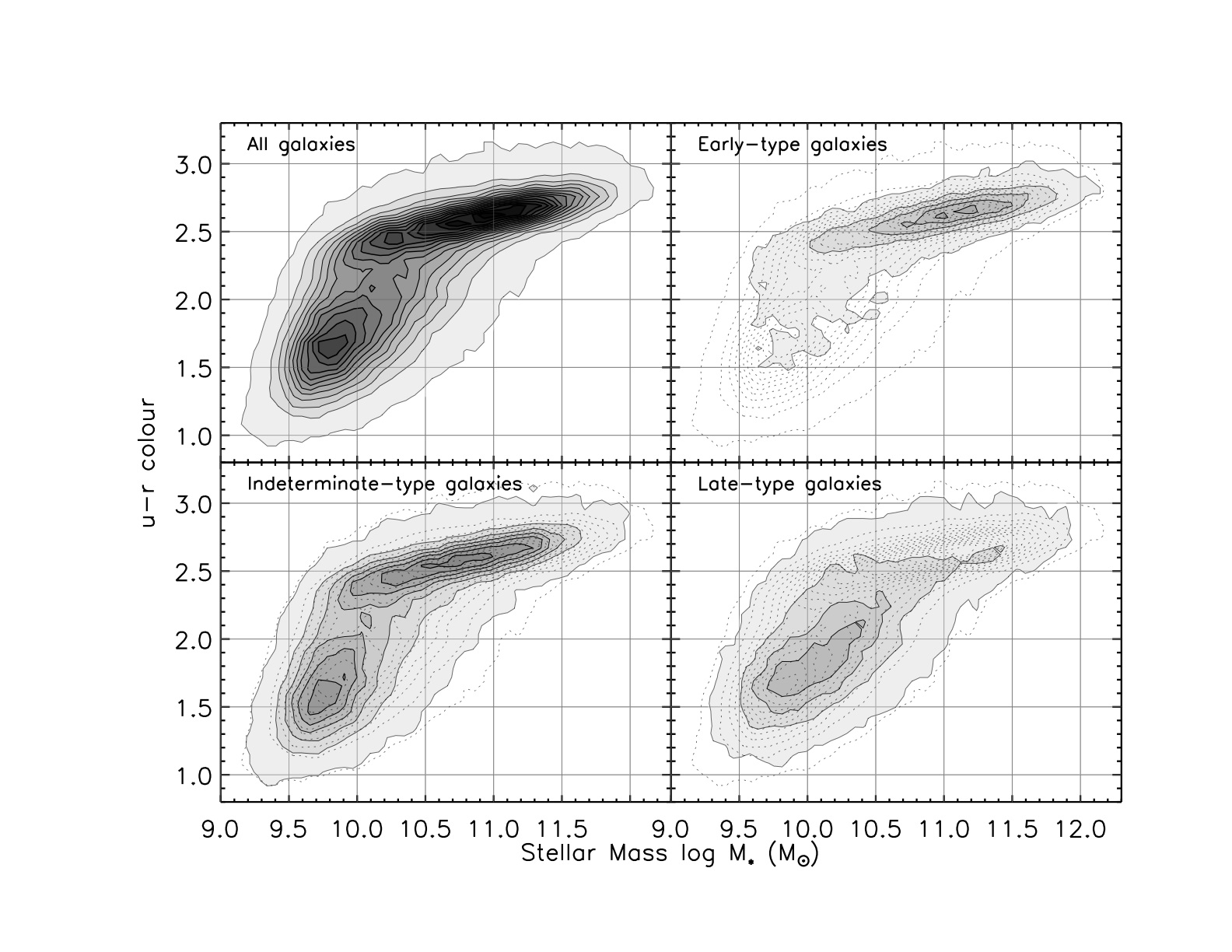
The color bimodality is similar to the morphologcal dichotomy (E/S0 versus spiral/irregular), but not identical. There exist populations of blue early-type galaxies and red spirals, with blue ellipticals most numerous in low-density environments and red spirals just outside the densest regions (Bamford et al. 2009 MNRAS 339, 1324). The "green valley" is too sparse for many red galaxies to become blue by adding starbursts; it is potentially very important that these galaxies in transition have the highest probability of hosting AGN.
An important description of the distribution and occurrence of galaxies is the luminosity function Φ : Φ(L) dL is the number of galaxies in the interval L +/- dL/2 per unit volume. This may be defined for optical luminosity, radio power, far-IR power, ... One always has the hope that this function is fundamental in telling how galaxy masses are distributed; that is, that all kinds of galaxies have about the same visible to invisible mass ratio. The determination of Φ over a wide luminosity range is complicated by Malmquist bias, and the need to reduce all measurements to a common emitted-wavelength frame - this is a special problem for QSOs and very luminous galaxies, for which we must look to significant redshifts to see any of the brightest examples. The luminosity function may be determined, in principle, very simply; for objects in luminosity bin i, the luminosity function is simply
Φ(Li ) = Σ (1/Vm)where Vm is the volume within which each object could have been detected, and the sum runs over all objects in bin i. All the selection effects fall into determining Vm for a given threshold condition, which may be nontrivial. Actually, it always seems to be nontrivial. An important application of Vmis the Schmidt V/Vm test, which can show whether the sample is complete or at least uniform, and can show the presence of some kinds of evolution with cosmic time when applied over a large redshift range. If the objects are uniformly distributed within the survey volume, the sample mean of the statistic V/Vm, where V is the volume of a sphere centered here and with the object at its surface, will be 1/2. [For cosmological applications one must worry about whether this is the right prescription for the volume of the sphere, integrating volume elements to the distance in question.] A value smaller than this implies that there are more objects close to us, which for galaxies normally means that the sample is more incomplete at large distances than we initially assumed. A mean value greater than 1/2 almost always implies cosmological evolution, as for QSOs. The fact that gamma-ray bursts show a value significantly smaller than 1/2 even for the most complete flux samples is one of their major puzzles.
From the magnitude-limited RSA catalog, the redshift distribution of catalog entries is shown here (less a single object at 9875 km/s).
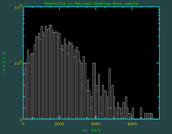
From the wide range of cz we see that the volumes sampled at various luminosities differ by factors of order 106. Thus careful allowances for sample properties is crucial to measuring the LF. This is clear when comparing the distribution of apparent and absolute magnitude shown in the figures below (again from the RSA, skipping three naked-eye members of the Local Group):

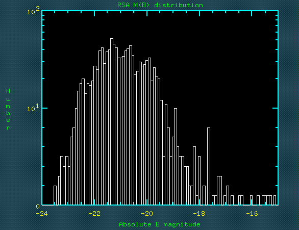
To derive the proper relative numbers, one must correct for the different volumes within which each object would appear in the catalog. This apparent distribution declines fainter than absolute blue magnitude -21.5, while the space density continues to increase greatly to fainter absolute magnitudes.
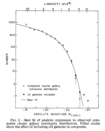 An important analytic approximation
to the overall galaxy luminosity
function is the Schechter (1976, ApJ 203, 297) form
Φ (L) dL =
φ* (L/L*)
α
e-(L/L*) (dL/L*)
where φ
*
(L/L*) is the normalizing factor, set by the number of galaxies
per Mpc3,
L* is a characteristic luminosity, and
α is an
asymptotic slope to be fit; a value around -5/4 usually agrees with the
data. The plot (from Schechter's paper, reproduced by permission of the AAS)
shows the fit to the mean of galaxy counts in 13 clusters.
An important analytic approximation
to the overall galaxy luminosity
function is the Schechter (1976, ApJ 203, 297) form
Φ (L) dL =
φ* (L/L*)
α
e-(L/L*) (dL/L*)
where φ
*
(L/L*) is the normalizing factor, set by the number of galaxies
per Mpc3,
L* is a characteristic luminosity, and
α is an
asymptotic slope to be fit; a value around -5/4 usually agrees with the
data. The plot (from Schechter's paper, reproduced by permission of the AAS)
shows the fit to the mean of galaxy counts in 13 clusters.
Different kinds of galaxies have different LF shapes and normlizations; this explains why Hubble thought of the LF as approximately Gaussian, from studies of (giant) spirals, while Zwicky counted everything, dissented vigorously and as usual correctly, and found a divergence at faint magnitudes. Zwicky distinguished dwarf, pygmy, and gnome galaxies (see his idiosyncratic book Morphological Astronomy). The LF must converge somewhere to avoid Olbers' paradox. The LF is simple only for dwarfs; the various types are distributed in Virgo as follows, from Fig. 1 of Binggeli, Sandage, and Tammann 1988 (Ann. Rev. 26, 509 - an excellent reference for the whole topic, figure reproduced from the ADS).
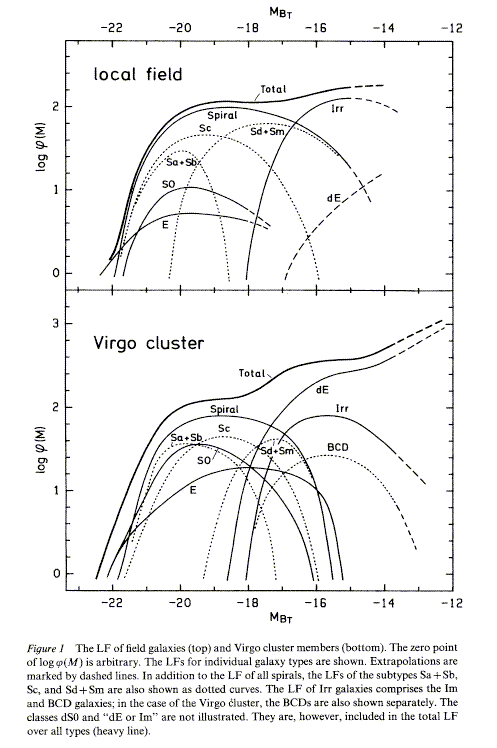
The differences may be clues to how different galaxy types form - in some biassing schemes, for example, ellipticals need stronger peaks than disks. On the other hand, if merging is important, this may tell us about the history of mergers rather than galaxy formation. It does seem to be quite consistent in shape among clusters of galaxies, so that it tells something basic and general about how galaxies have developed.
Similar clues are hidden in some of the basic correlations among global galaxy properties involving dynamics - the Tully-Fisher and Faber-Jackson relations. The Tully-Fisher relation, often employed as a distance indicator for spirals, is a tight relation between galaxy absolute magnitude and velocity scale of the disk (for example, at the 20% - of - peak level in an integrated H I profile, with appropriate inclination corrections). There are broad theoretical reasons why such a relation might hold, but no deep understanding at this point. The Faber-Jackson relation was also found empirically, from the fact that elliptical-galaxy luminosity and central velocity dispersion σ are related approximately as L ~ σ 4. A generalization, the fundamental plane, was found by noting that scatter about the F-J relation is correlated with metallicity (usually through a simple index of Mg absorption), although it turned out that this may not be the most basic parametrization. Not only is the fundamental plane a useful distance and environment probe, but it sets strong constraints on dynamical evolution; any transformations of galaxies must leave them very close to this plane. Since (in log space) the fundamental plane is, as far as we can tell, a plane, there are transformations of variables which correspond to orthogonal variables imbedded in it; Burstein and coworkers have explored the interpretation of these so-called κ parameters.
Basics of the "fundamental plane" may be found in the review by Kormendy and Djorgovski (1989, ARA&A 27, 235). Their Figure 2 (reproduced from the ADS) compares the observed Faber-Jackson relation (upper left) to more exact projections of the galaxy distribution in the volume of radius, surface brightness, and velocity dispersion.
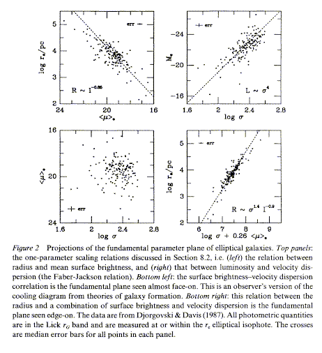
In the observable parameters, R ~ σ 1.4 +/- 0.15 I-0.9 +/- 0.1 where R is an effective or core (but not isophotal) radius, σ is the velocity dispersion (one-dimensional, in the line of sight), and I is an averaged intensity (commonly the mean within the effective radius). Some of the earlier relations, such as L ~ σ 4 and Dn ~ σ 4/3 for diameter to reach a particular mean surface brightness, are projections of this plane along different observable axes. One mapping of particular theoretical interest (in which galaxies are widely spread) is the &sigma - μ plane, corresponding roughly to the density - cooling rate prescription needed to describe a galaxy's initial collapse. The virial theorem suggests a relation of about the FP form, with departures of the scaling exponents from 2 and 1 coming about if there is systematic variation in the (M/L) ratio with luminosity or other global parameters. The narrowness of the fundamental plane tells us that evolution by merging, if it is significant for ellipticals, must carry galaxies along but not across the plane. There are simulations suggesting that the FP parameters are indeed preserved during (some kinds of) merging. Recent work indicates the the fundamental plane shifts at least in luminosity with redshift, as expected for a broad class of galaxy-evolution schemes.
Last changes: 8/2009 © 2000-2009